Palmer Lab

Location and Contact Information
630 W. 168th Street
Black Building, Room 511
New York, NY 10032
United States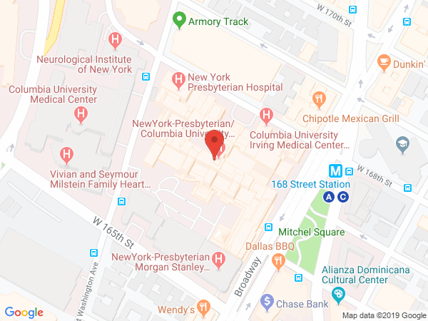
Principal Investigator

The Palmer Laboratory in the Department of Biochemistry and Molecular Biophysics uses NMR spectroscopy to study the structures and dynamical properties of proteins and other macromolecules.
Publications
Lab Members